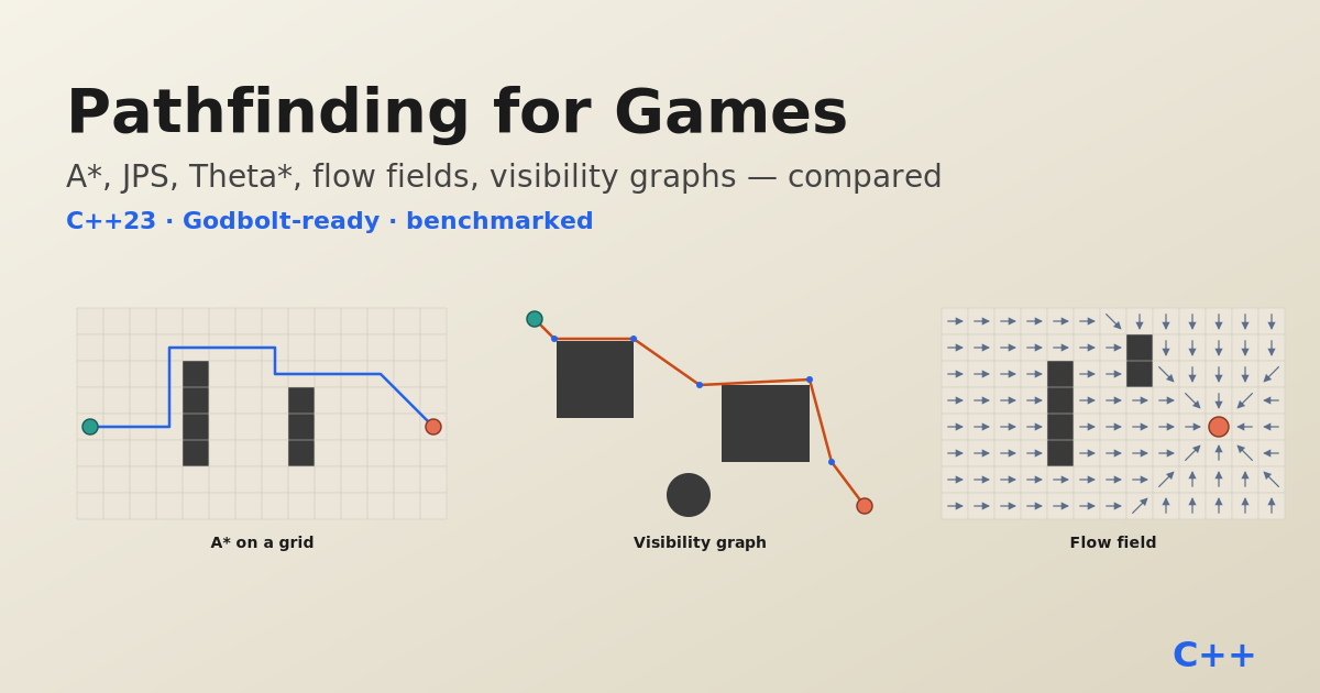
I watched Raymi Klingers’ Meeting C++ 2025 talk Age of Empires: 25+ years of pathfinding problems with C++ last week and came away with two thoughts. First: pathfinding is a 40-year-old problem that still ships with fresh bugs in modern game engines. Second: nobody writes a single post that lines up the actual algorithms — A*, JPS, Theta*, flow fields, visibility graphs — with code you can paste into Godbolt and benchmarks that let you reason about tradeoffs.
So I wrote one.
Every implementation below is a single C++23 translation unit, no dependencies, builds with -O2 -std=c++23 on GCC 14. Every code block has a Godbolt link. The same grid generator feeds all of them so the numbers are directly comparable. I ran everything in Docker on gcc:14 and the results section is what actually came out of my machine, not what a paper’s abstract promised.
Why pathfinding is still hard
Three structural pressures make game pathfinding a different problem from textbook shortest-path:
- Wall-clock budget. You have a few milliseconds per frame shared across every system. A 500-unit RTS needs 500 paths computed, updated, and replanned per second — without blowing the frame budget.
- Dynamic obstacles. Other units move. Buildings get placed and destroyed. A path is a hypothesis that expires.
- Predicates that disagree with themselves. This is the Klingers/AoE punchline.
orient2d(a,b,c)with floats + SIMD + no x87 extended precision can return different signs depending on evaluation order. Units phase through buildings. Integer arithmetic fixes it.
Grid A* handles some of these; none of them well. The field has accumulated half a dozen specialised approaches, each with a tight win condition.
A* — the baseline
Nothing beats A* at being obvious. Expand the open-set node with minimum f(n) = g(n) + h(n), where g is the cost so far and h is an admissible heuristic (for 8-connected grids, octile distance: 10*(dx+dy) + (14-20)*min(dx,dy) with straight-cost 10 and diagonal 14).
The only subtlety worth calling out: corner rules. Three policies are in common use:
- Free corner cutting — diagonals always allowed. Paths get through single-cell gaps; feels “wrong” visually.
- No squeeze — diagonal allowed unless both adjacent cardinals are blocked. What the JPS paper assumes.
- No corner cut — diagonal allowed only if both cardinals are walkable. What most RTS games ship.
The “no squeeze” rule is used throughout this post. It matters: mismatched rules between A* and JPS is a silent source of bugs where one algorithm reports a shorter cost than the other. Ask me how I know.
[[nodiscard]] AStarResult astar(const Grid& g, Point s, Point t) {
    struct QI { int f, x, y;
        constexpr bool operator<(const QI& o) const noexcept { return f > o.f; } };
    std::priority_queue<QI> open;
    std::vector<int> gcost(g.W * g.H, INT32_MAX);
    std::vector<int> parent(g.W * g.H, -1);
    std::vector<std::uint8_t> closed(g.W * g.H, 0);

    gcost[s.y * g.W + s.x] = 0;
    open.push({octile(s.x, s.y, t.x, t.y), s.x, s.y});

    while (!open.empty()) {
        auto [f, x, y] = open.top(); open.pop();
        if (closed[y * g.W + x]) continue;
        closed[y * g.W + x] = 1;
        if (x == t.x && y == t.y) [[unlikely]] { /* reconstruct */ return r; }
        for (std::size_t i = 0; i < 8; ++i) {
            int nx = x + DX[i], ny = y + DY[i];
            if (!g.walkable(nx, ny)) continue;
            if (i >= 4 && !g.walkable(x+DX[i], y) && !g.walkable(x, y+DY[i])) continue;
            int ng = gcost[y * g.W + x] + DC[i];
            if (ng < gcost[ny * g.W + nx]) {
                gcost[ny * g.W + nx] = ng;
                parent[ny * g.W + nx] = y * g.W + x;
                open.push({ng + octile(nx, ny, t.x, t.y), nx, ny});
            }
        }
    }
    return r;
}
The C++23 niceties that actually help: [[nodiscard]], std::println instead of printf, designated initializers for the Grid{.W=W, .H=H, ...} ctor, std::ranges::reverse on the reconstructed path.
Godbolt: full astar.cpp with scenarios · gcc 14.3, -O2 -std=c++23.
Jump Point Search — and why it’s often slower
JPS (Harabor & Grastien, AAAI 2011) is A*’s younger, more aggressive sibling. It assumes a uniform-cost 8-connected grid and exploits the fact that most of A*’s open-set pushes are symmetric — different paths of equal length expanded into the open list. JPS prunes symmetric paths by “jumping” in straight lines until it finds a reason to stop.
The stop conditions are:
- The ray hits a blocked cell or the edge of the grid → abort.
- The ray reaches the goal → success.
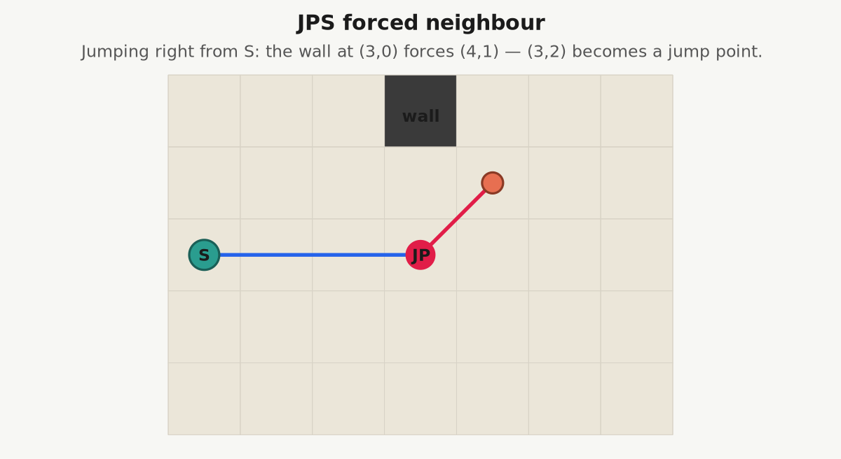
- The current cell has a forced neighbour — a neighbour A* would have considered because an obstacle elsewhere makes that neighbour not-symmetric. This cell is a jump point. Add it to the open set.
- For diagonal rays, recurse along the two cardinal components; if either finds a jump point, the current cell is a jump point.
The bug I hit
My first JPS implementation reported an 8-unit-shorter optimal cost than A* on the same grid. Classic symptom of squeezing through a pinch. The fix is subtle:
[[nodiscard]] static bool jump(const Grid& g, int x, int y, int dx, int dy,
                               int tx, int ty, int& ox, int& oy) {
    while (true) {
        int nx = x + dx, ny = y + dy;
        if (!g.walkable(nx, ny)) return false;
        // No-squeeze must be checked BEFORE declaring (nx,ny) as anything.
        if (dx != 0 && dy != 0
            && !g.walkable(nx - dx, ny) && !g.walkable(nx, ny - dy))
            return false;
        if (nx == tx && ny == ty) { ox = nx; oy = ny; return true; }
        // ... forced-neighbour checks ...
    }
}
If the squeeze check comes after the forced-neighbour check, you can return a jump point that you couldn’t actually have stepped to. The diagonal move needs to be legal first, then we ask whether it’s a jump point. Got the order backwards once, paid for it with a verifier that caught the illegal step (18,5)→(19,6) — both (18,6) and (19,5) blocked.
When does JPS actually win?
In the benchmark below, naive recursive JPS on a 512x512 rooms-and-corridors map expands 22x fewer nodes than A — and runs 2.5x slower*. The recursion cost in the inner loop eats the savings. This is not a new observation; it’s why JPS+ exists (Harabor & Grastien, ICAPS 2014) — JPS with offline preprocessing of all jump points — and why Steve Rabin’s GDC JPS+ work produces the production-grade speedup people cite. Treat naive JPS as the algorithm, JPS+ as the implementation that ships.
Godbolt: full jps.cpp.
Theta* — any-angle paths
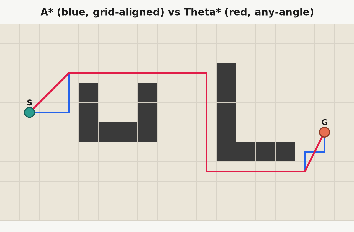
A* produces grid-aligned zigzags. Post-smoothing helps but is a hack layered on top of a wrong answer. Theta* (Nash, Daniel, Koenig, Felner, AAAI 2007) fixes it at the source: on each relaxation, check whether the current node’s grandparent has line-of-sight to the neighbour. If yes, skip the current node and use the grandparent as the parent directly. The result is a path that hugs obstacle corners along straight segments.
// Path-2: grandparent has LOS to the neighbour.
if (line_of_sight(g, gpP, {nx, ny})) {
    ng = gcost[gp] + euclid(gpP.x, gpP.y, nx, ny);
    np = gp;
} else {
    // Path-1: classic A* relaxation.
    double step = (i < 4) ? 1.0 : std::sqrt(2.0);
    ng = gcost[idx(x, y)] + step;
    np = idx(x, y);
}
The LOS check is Bresenham with a no-squeeze guard at diagonal steps. Every relaxation pays an O(grid-diagonal) LOS cost, which is why Theta* expands as many nodes as A* but runs 2–8x slower in wall time. The payoff: paths that are 2–3% shorter in Euclidean distance and look dramatically better (12 waypoints instead of 50).
Theta* is the right call when path quality matters more than solve time — ships, tanks, vehicles in big open spaces. It’s the wrong call for swarms of units where visual smoothing is done by steering anyway.
Godbolt: full theta.cpp.
Flow fields — one Dijkstra, a thousand agents
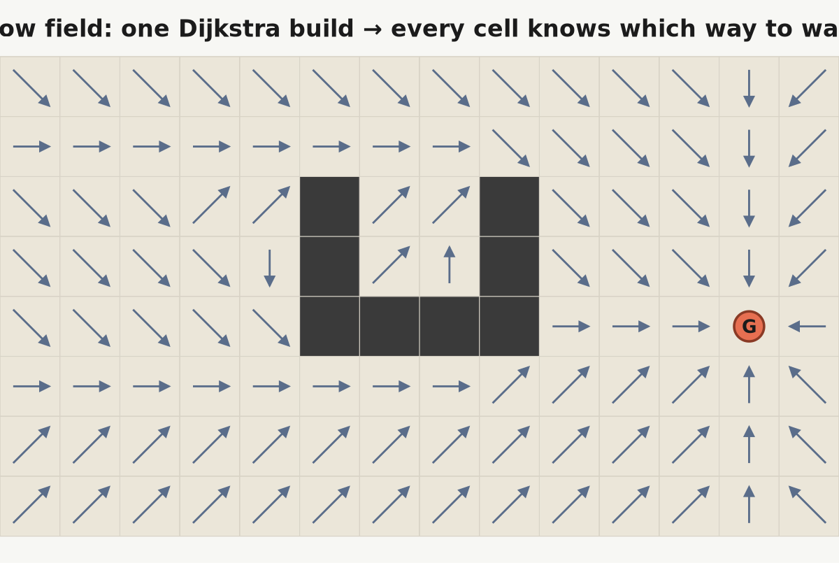
A* and JPS amortise poorly across agents: each agent gets its own search. Elijah Emerson’s “Crowd Pathfinding and Steering Using Flow Field Tiles” (Game AI Pro, ch. 23) flips the problem: if 500 marines are all moving to the same mineral field, do one reverse Dijkstra from the goal. Store two fields:
- Integration field — 32-bit cost-to-goal per cell.
- Flow field — 8-bit direction index (0..7 for the eight neighbours, -1 for unreachable).
Every agent reads its cell’s flow index, steps, repeats. Build cost O(V log V); per-agent query O(1).
[[nodiscard]] static FlowField build_flow_field(const Grid& g, Point goal) {
    FlowField ff{/* ... */};
    std::priority_queue<QI> pq;
    ff.integration[idx(goal.x, goal.y)] = 0;
    pq.push({0, goal.x, goal.y});

    while (!pq.empty()) {
        auto [d, x, y] = pq.top(); pq.pop();
        if (d > ff.integration[idx(x, y)]) continue;
        for (std::size_t i = 0; i < 8; ++i) {
            int nx = x + DX[i], ny = y + DY[i];
            if (!g.walkable(nx, ny)) continue;
            if (i >= 4 && !g.walkable(x+DX[i], y) && !g.walkable(x, y+DY[i])) continue;
            std::int32_t nd = d + DC[i];
            if (nd < ff.integration[idx(nx, ny)]) {
                ff.integration[idx(nx, ny)] = nd;
                pq.push({nd, nx, ny});
            }
        }
    }
    // Second pass: flow = argmin over 8 neighbours of integration.
    // ...
    return ff;
}
On my 512x512 random map: flow-field build takes 45ms, but following it for 1000 agents costs 5.7 µs/agent. A* over the same map costs 8.6ms per query × 1000 agents = 8.6 seconds. Flow fields break even vs per-agent A* at roughly 5 agents sharing a goal.
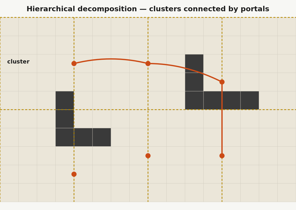
Supreme Commander 2 took this further with sector-portal decomposition — the map is split into 10×10-cell sectors, A* runs on the portal graph, flow fields are computed lazily per (portal window, goal). Emerson’s chapter is the canonical reference and worth reading in full.
Godbolt: full flowfield.cpp.
Visibility graphs — the AoE II DE approach
AoE II DE’s short-range pather uses a different primitive entirely. Obstructions are circles (units, trees) and AABBs (buildings). Instead of pathing on a grid, expose the hull vertices of each obstruction — corners for boxes, sampled tangent points for circles — then:
- Build a graph over all mutually-visible vertex pairs + start + goal.
- Drop edges that intersect any obstruction interior.
- A* over the resulting graph.
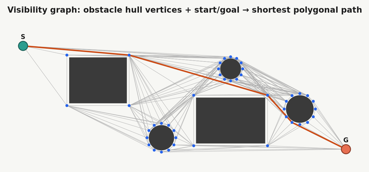
The graph stays small (a few hundred vertices for typical obstacle counts), and the resulting path is optimal among polygonal paths — and naturally tangent to obstacles.
The interesting engineering problem isn’t the search. It’s the geometric predicates:
// Orient2d in 64 bits — exact for 8.8 fixed-point inputs on maps up to ~32k tiles.
[[nodiscard]] constexpr std::int64_t orient2d(Pt a, Pt b, Pt c) noexcept {
    const std::int64_t abx = std::int64_t(b.x.v) - a.x.v;
    const std::int64_t aby = std::int64_t(b.y.v) - a.y.v;
    const std::int64_t acx = std::int64_t(c.x.v) - a.x.v;
    const std::int64_t acy = std::int64_t(c.y.v) - a.y.v;
    return abx * acy - aby * acx;
}
This is the punchline of Klingers’ talk. When Forgotten Empires modernized AoE II and compilers enabled SIMD by default, two things happened simultaneously: denormals started flushing to zero, and 80-bit x87 extended precision went away on x64. Geometric predicates that used to classify points consistently started disagreeing with themselves depending on evaluation order. Units phased through buildings. The fix was to move to 8.8 fixed-point coordinates and integer predicates. orient2d now returns int64_t; segment-vs-circle uses __int128 to avoid overflow. Same inputs, same output, every compiler flag, every hardware target.
The talk calls this a self-verifiable algorithm. That’s the right framing. A floating-point predicate is a heuristic that happens to be right most of the time. An integer predicate is a theorem.
Godbolt: full visibility.cpp.
Sidebar: StarCraft: Brood War’s pathfinding
Patrick Wyatt (BW lead programmer) wrote The StarCraft path-finding hack — the canonical primary source. The structure:
- Regions — static on map load, ~10×10 terrain tiles each, used as nodes for high-level A*.
- Walk tiles — 8×8-pixel grid for low-level movement. Warcraft had 32×32 tiles with 16 sub-cells; StarCraft bumped to 8×8 because of isometric art, inflating the pathing map 16×.
- Local collision — a “gigantic state-machine which encoded all sorts of specialized ‘get me out of here’ hacks.” Units that couldn’t resolve a collision just stopped. Hence the Dragoon’s famous reputation for failing to path — it was the largest ground unit and got wedged most often.
And the shipping hack: “whenever harvesters are on their way to get minerals, or when they’re on the way back carrying those minerals, they ignore collisions with other units.” That’s why idle harvesters spread out when you stop them — they finally start checking tiles. No flow fields, no navmesh, just regions + 8×8 grid A* + a collision-avoidance state machine with escape hatches.
BWAPI exposes the region graph via BWAPI::Region. For a clean C++ reimplementation of the original engine with the pathing preserved, see OpenBW. Terrain-analysis libraries like BWTA do their own Voronoi-based region decomposition — useful if you want the abstract structure without reading Blizzard’s original bytes.
What StarCraft 2 changed
Anhalt, Kring, and Sturtevant presented the SC2 architecture at GDC 2011 — “AI Navigation: It’s Not a Solved Problem Yet”. Three layers:
- Constrained Delaunay triangulation navmesh — runtime representation, separate layers for ground, flying, cliff-transitions.
- A over the triangulated graph* — with “tunnel” portals between adjacent triangles.
- Steering behaviours — Boids-style, with horizon analysis predicting collisions before they happen.
Group movement uses flow fields over the navmesh. The net effect: no BW-style deadlock. Units push and slide around each other rather than stopping and waiting for a timeout.
This is the template most modern engines follow. Unreal’s navmesh is Recast/Detour. Unity’s AI Navigation package is Detour. Godot’s navigation server uses Recast for baking. The navmesh has won.
Benchmarks
One combined binary that runs all four grid algorithms on identical scenarios. Same RNG seeds, same start/goal, same corner rule.
Source: bench.cpp on Godbolt.
=== Random 20% blocked (512x512) ===
algo              nodes    cost(x10)    time (us)
A*                32718         7526         8650
JPS               30831         7526        14144
Flow             209433         7526        24685   full field, any goal
Theta*            37702         7351        20916   any-angle Euclidean

=== Rooms and corridors (512x512) ===
algo              nodes    cost(x10)    time (us)
A*                58657         7774         9664
JPS                2653         7774        24448
Flow             255361         7774        26348   full field, any goal
Theta*            58252         7497        77186   any-angle Euclidean

=== Random 15% blocked (1024x1024) ===
algo              nodes    cost(x10)    time (us)
A*                87713        14772        19817
JPS               85311        14772        48358
Flow             890992        14772       112191   full field, any goal
Theta*           118544        14570        85951   any-angle Euclidean
All costs are scaled by 10 so octile and Euclidean stay comparable. Key readings:
- All four agree on octile-optimal cost (7526, 7774, 14772) when measuring grid-edge paths. Only Theta*’s Euclidean cost is strictly shorter — because it’s not restricted to grid edges.
- A wins wall time in every scenario.* On random maps, JPS expands almost as many nodes (JPS’s advantage is open corridors). On rooms, JPS expands 22x fewer nodes — but its per-jump work dominates.
- Flow field’s build cost scales with reachable cells, not path length. On the 1024² map it fills the entire reachable component (890k cells). The win comes from amortising that build across many agents, not from single-path latency.
- Theta’s LOS checks are expensive in open rooms.* 77ms vs A*’s 9.7ms — 8x slower — for a path 3.6% shorter. For most games this isn’t worth it. For a ship that turns slowly, it is.
Why naive JPS loses wall time
Two reasons, both implementation-level:
- Recursion. Each diagonal step makes two recursive cardinal jumps. In open rooms those cardinal jumps can scan 64 cells at a time. You save on open-set pushes but pay in cell visits.
g.walkable()has a bounds check. With-O2it inlines but the branch is still there. Production JPS uses sentinel borders (pad the grid with an extra row/column of blocked cells) so the bounds check can be removed.
JPS+ avoids both by precomputing the jump distance from every cell in every direction. Inner loop becomes a table lookup. This is also why the GPPC (Grid Pathfinding Competition) leaderboards are dominated by JPS+ variants: the win is in the preprocessing, not the online algorithm.
Which one should you pick?
| Scenario | Use |
|---|---|
| Single agent, uniform-cost grid, small map | A* — it’s the baseline and it’s good enough |
| Single agent, large mostly-open grid, offline preprocessing OK | JPS+ |
| Hundreds of agents, same goal | Flow field |
| Large open 3D world with dynamic obstacles | Navmesh (Recast/Detour) |
| Path aesthetics matter (ships, vehicles, cinematics) | Theta* |
| Few obstructions but exact geometry needed (AoE-style buildings + units) | Visibility graph with integer predicates |
| Many agents, varying goals, tight frame budget | Hierarchical (HPA*/regions + local A*) |
Libraries and reference implementations
Worth linking over rewriting:
Navigation meshes
- recastnavigation/recastnavigation — Mikko Mononen’s navmesh toolkit. Ships inside Unreal; wrapped by Unity AI Navigation and Godot.
JPS and any-angle search
- nathansttt/hog2 — Nathan Sturtevant’s C++ testbed: A*, JPS, JPS+, Theta*, HPA*, with loaders for Baldur’s Gate / Dragon Age / StarCraft benchmark maps.
- KumarRobotics/jps3d — UPenn’s C++ 2D/3D JPS, robotics-grade.
- PathPlanning/AStar-JPS-ThetaStar — clean academic C++ implementation of the three-paper triple.
- qiao/PathFinding.js — JS, but the best-annotated JPS reference. Good for reading.
Benchmarks
- movingai.com/benchmarks — Sturtevant’s grid-pathfinding benchmark set, used by every serious pathfinding paper.
- GPPC — the annual Grid Pathfinding Competition at ICAPS/AAAI.
StarCraft
- bwapi/bwapi — Brood War API, the base for BW bot research.
- OpenBW/openbw — open-source BW engine reimplementation that preserves the original (buggy) pathfinding.
HPA and flow fields*
- hugoscurti/hierarchical-pathfinding — closest to a reference HPA* implementation, tested on Dragon Age maps.
- vonWolfehaus/flow-field — the canonical “flow field + steering” demo people cite after the Planetary Annihilation GDC talk.
Engine source
- godotengine/godot —
modules/navigation/wraps Recast for baking; runtime NavigationServer is original.
All Godbolt links
Everything above is paste-and-compile:
| File | Description | Link |
|---|---|---|
astar.cpp | Grid A* baseline, C++23 | godbolt.org/z/hzhGcYdjz |
jps.cpp | Jump Point Search (naive recursive) | godbolt.org/z/df7YK49fM |
flowfield.cpp | Reverse-Dijkstra flow field + follower | godbolt.org/z/8E45dTWvc |
theta.cpp | Theta* any-angle with Bresenham LOS | godbolt.org/z/M8YdxYbcz |
visibility.cpp | AoE-style visibility graph, fixed-point predicates | godbolt.org/z/75brG4E8E |
bench.cpp | All four grid algorithms in one binary | godbolt.org/z/4K7h8E1xG |
All compile with GCC 14.3, -O2 -std=c++23. The main C++23 features in use are std::print/std::println (cleaner than printf), [[nodiscard]] on search-result types, designated initializers for struct ctors, and std::ranges::reverse. Nothing exotic — the algorithms would look nearly identical in C++17. C++23 just makes the scaffolding quieter.
Further reading
- Klingers, R. “Age of Empires: 25+ Years of Pathfinding Problems with C++,” Meeting C++ 2025.
- Harabor, D.; Grastien, A. “Online Graph Pruning for Pathfinding on Grid Maps,” AAAI 2011 (JPS).
- Nash, A.; Daniel, K.; Koenig, S.; Felner, A. “Theta*: Any-Angle Path Planning on Grids,” AAAI 2007.
- Emerson, E. “Crowd Pathfinding and Steering Using Flow Field Tiles,” Game AI Pro ch. 23, CRC Press 2015.
- Botea, A.; Müller, M.; Schaeffer, J. “Near Optimal Hierarchical Path-Finding,” Journal of Game Development, 2004 (HPA*).
- Wyatt, P. “The StarCraft Path-Finding Hack,” Code of Honor blog, 2013.
- Anhalt, J.; Kring, K.; Sturtevant, N. “AI Navigation: It’s Not a Solved Problem Yet,” GDC 2011 (SC2).
- Patel, A. “Introduction to A*,” Red Blob Games. Still the best first read.
The punchline I keep coming back to: pathfinding is not one algorithm. It’s a portfolio. Pick the piece that matches the actual constraint — agent count, map density, solve-time budget, whether path aesthetics matter. Then ship something you can verify. Integer predicates if you care whether your units stay on the right side of a wall. Benchmarks if you care whether it runs in your frame.